Linear Classifiers

In this post we will discuss linear classifiers a type of machine learning algorithm , we’ll start by discussing linear classifiers for two classes , then talk about logistic regression for classification , a particular type of linear classifier. For an introduction to classification and other types of classifiers check out my post on K-nearest Neighbors for classification, but lets quickly review the classification problem.

There are two parts to the classification problem , the labels and features. The features are usually numeric values or simply vectors, and classes are discrete values. We can plot out the features and use colors to represent each label . For example we have three samples with three different classes green, blue and red. The first sample x₁ has a value of 4 and belongs to the red class as shown in Figure 1. Similarly, if sample x₂ had a value of 1 and belonged to the blue class we would plot the point as shown in figure 1 . Sample x₃ belongs to the green class and has a value of zero as shown if figure 1 .

*Fig 1 Three samples* x₁, x₂ *and* x₃ *on points three, one and zero respectively, each sample has it’s class color overlaid on the point*

We can use the variable y to represent the class this is shown in figure 2 where we have three samples x₁, x₂ and x₃ plotted in two dimensions. The variable y₁, y₂ and y₃ has a class value of zero, one and two respectively. We overlay the class color over the points as shown in figure 2 . Lets focus on the two class problem.

*Fig 2 Three samples* x₁, x₂ *and* x₃ *on points three, one and zero respectively, each sample has it’s class color overlaid on the point*.

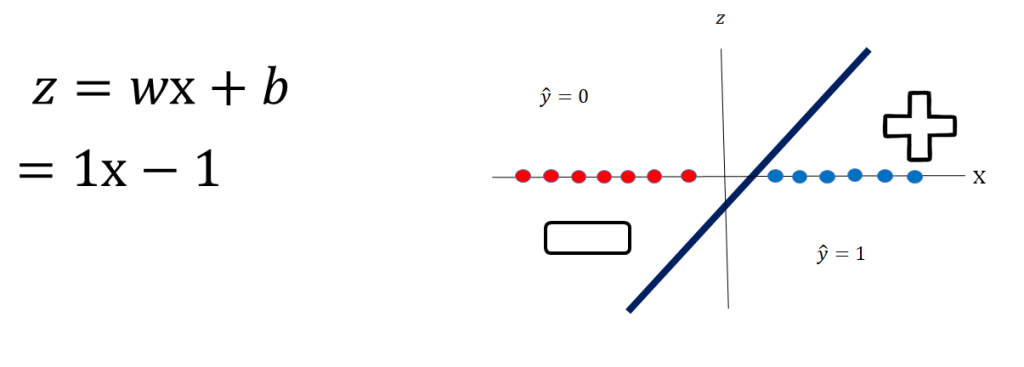
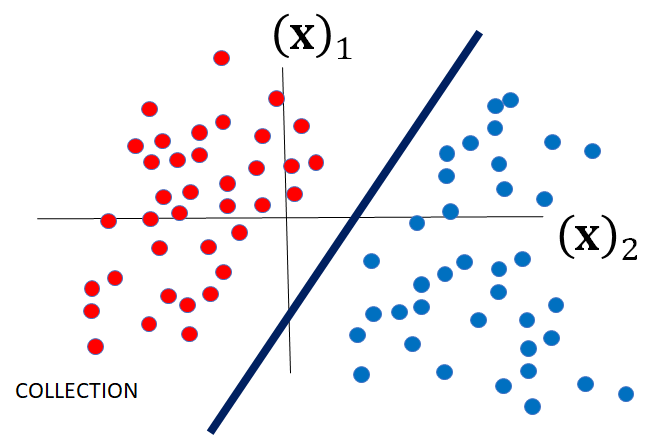
Examining figure 3 we have two different classes. Class zero is denoted in red and class one is denoted in blue. Examining the figure we can see that we can separate the classes by using a vertical line.

Fig 3: two class classification red points represent points where the value of the class y=0 and

Let’s look at the equation of a line i.e. z=x -1 as shown in figer 4. If c will be negative. Thus, if a data set can be separated by a line the data set is said to be linearly separable. Let’s verify this with an example.

Fig 4: example of a line z=x-1 if x on the right side of the line, the value of z will be positive , if we pick a value of x on the left side of the line, the value of z will be negative

Let’s select the value of x to be 3. We plug it into the equation of our line and find that the value of z is 2. As shown in Figure 5:

Fig 5: setting a value of x=3 and plugging it into the equation of the line the value of z is 2.

Let’s try another example whit the red class ie y=0, Let’s say we choose the value of x to be -2. We plug it into the equation of our line and find that the value of Z is -3 as shown in figer 6.

*Fig 6: setting a value of x=-2 and plugging it into the equation of the line the value of z is* -3.

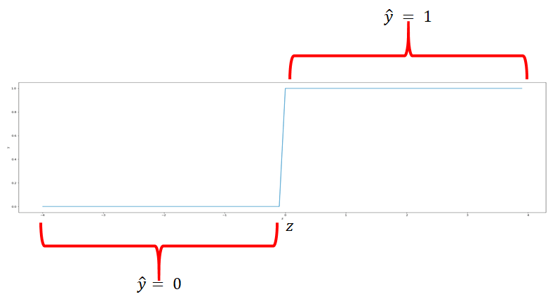
If we use this line to calculate the class of the points it always returns real numbers such as -1, 3, -2, and so on. But we need a class between 0 and 1. So how do we convert these numbers? We’ll use something called the threshold function. If z is greater than 0, the threshold function will return a 1, and if z is less than 0, the threshold will return a 0. The is shown if figure 7. Let’s see how the threshold function works in concert with the the line.

Fig 7: threshold function if the input z is greater than 0, it will return a 1, and if the input z is less than 0, it will return a 0.

Combining the threshold function if we plug in the value of x as 3 ; the value of z is 2, this is shown in figure 8. The value of z equals to 2; this is passed on to the threshold function as show on the top of figure 7, the result is $\hat{y}$ will be 1.

Fig 8: Combining the linear function and the threshold function plugging in the value of x as 3 ; the value of z is 2, this is intern passed through the threshold function giving a value of $\hat{y}$ to be 1.

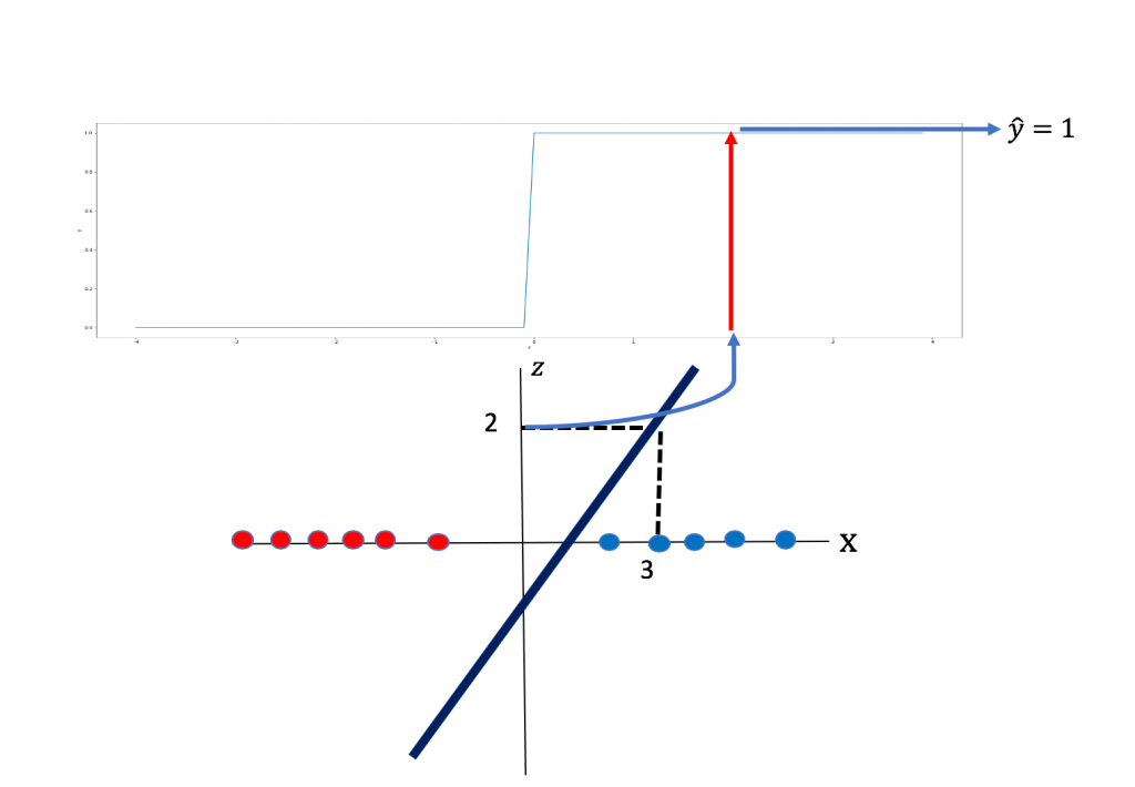Fig 8: Combining the linear function and the threshold function plugging in the value of x as 3 ; the value of z is 2, this is intern passed through the threshold function giving a value of $\hat{y}$ to be 1.

Similarly, If we plug in the value of x as -2, the value of z is -3. We pass through the threshold function and we get a 0. This is shown in figer 9:

Fig 9: Combining the linear function and the threshold function plugging in the value of x as -2 ; the value of z is -2, this is intern passed through the threshold function giving a value of $\hat{y}$ to be 0 .

Logistic Regression

Now let’s talk about logistic regression. The logistic function resembles the threshold function. The logistic function expression and the plot of the logistic function is shown in figure 10. The logistic function provides a measure of how likely a sample belongs to another class, in addition It has better performance then the threshold function for reasons we will discuss in another post . If the value of z is a very large negative number the value for the logistic function is approximately 0. For a very large positive value of z the value for the logistic function is approximately 1. And for everything in the middle the value is between 0 and 1 .

Fig 10: Logistic function expression and the plot of the logistic function.

To determine $\hat{y}$ as a discrete class we use a threshold shown by the line in figure 11 . If the output of the logistic function is larger than 0.5 we set the prediction value that to one, if it’s less we set it to $\hat{y}$ to 0. Let’s try out some values of x that we used previously with the linear classifier. Consider figure 11, if we set x equal to 3 in the equation of the line we get the value of z as 2. We pass it through the sigmoid function and since the value of the sigmoid function is greater than 0.5, we set that value of $\hat{y}$ to 1.

Fig 11: Combining the linear function, logistic *and the threshold* function plugging in the value of x as 3 ; the value of z is 2, this is intern passed through the logistic function then threshold function giving a value of $\hat{y}$ to be 1.

Similarly, If we plug in the value of x as -2 the value of z is -3. We pass the value of z through the sigmoid function we see the result is less than 0.5 so we set $\hat{y}$ to 0, this is shown in figer 12 .

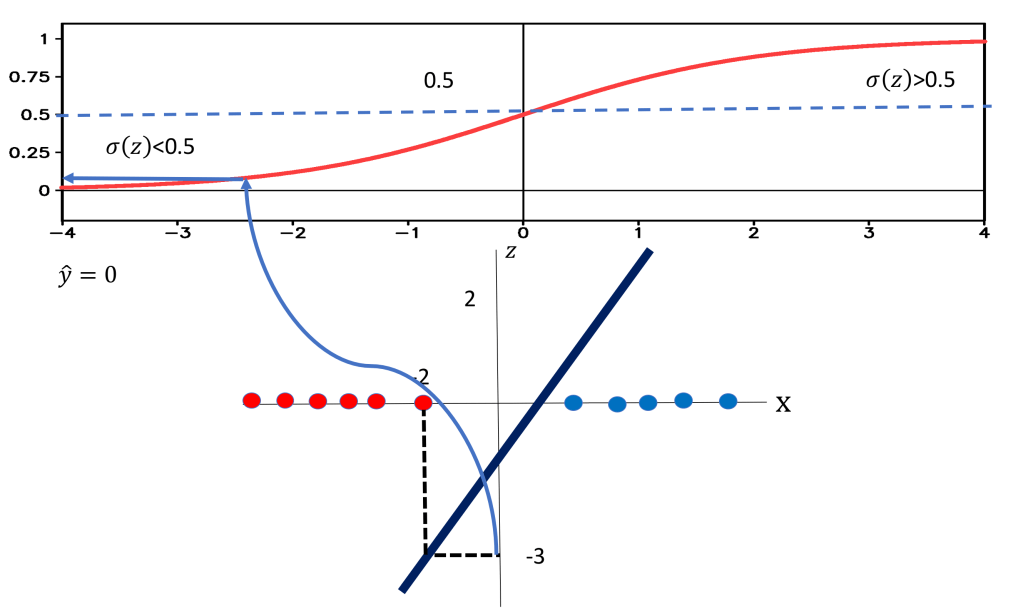Fig 12: Combining the linear function logistic and the threshold function plugging in the value of x as -2 ; the value of z is -2, this is intern passed through the threshold function giving a value of $\hat{y}$ to be 0 .

The output of the logistic function can provide a means of determining how confident you are about the classification. If the points are very close to the center of the separating line the value for the sigmoid function is very close to 0.5, this means that we are not certain if the class is correct. If the points are far away the value for the sigmoid function is either 0 or 1, respectively this means we are certain about the class. This is shown in figure 12 the points x₁ and x₂ are not close to the separating line a small change in either will cause them to change their class; as a result we our uncertain about the true class of the sample and the output of the sigmoid function is near 0.5 as shown in the first two rows of the table . Conversely x₃ and x₄ are relatively far away from the separating line as such the sigmoid function is near zero or one.

Fig 13 If the points are very close to the center of the line the value for the sigmoid function is very close to 0.5

Linear classifiers can be used for classifying samples in any dimension, lets look at the 2Dcase . Instead of a line to classify samples, we use a plane or hyperplane, this is shown in figure 13. If we look at a bird’s eye view of the plane we can get a better understanding of how the plane separates the data.

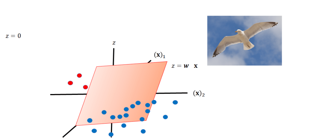
z equals 0, we can also see that as a line.We can visualize the plane at z = 0 as a line. This line can be used for separating the data, as shown in Fig 14.

Fig 14 *line separating data this is where the decision surface insects with the plane where z equals zero*

If you’re on one side of the plane you would get a negative value.Passing that into the threshold function Passing that into the threshold function you get a 0. as. shown in Fig . If you’re the other side of the plane, you would get a positive number, passing into the threshold function, you’ll get a one.

*Fig 15 line separating data this is where the decision surface insects with the plane where z equals zero*, the sample x₁ is produces a positive value, this intern is passed to the threshold function that outputs a one. The value of x₂ *is produces a negative value*, when this is passed into the threshold function we get a zero.

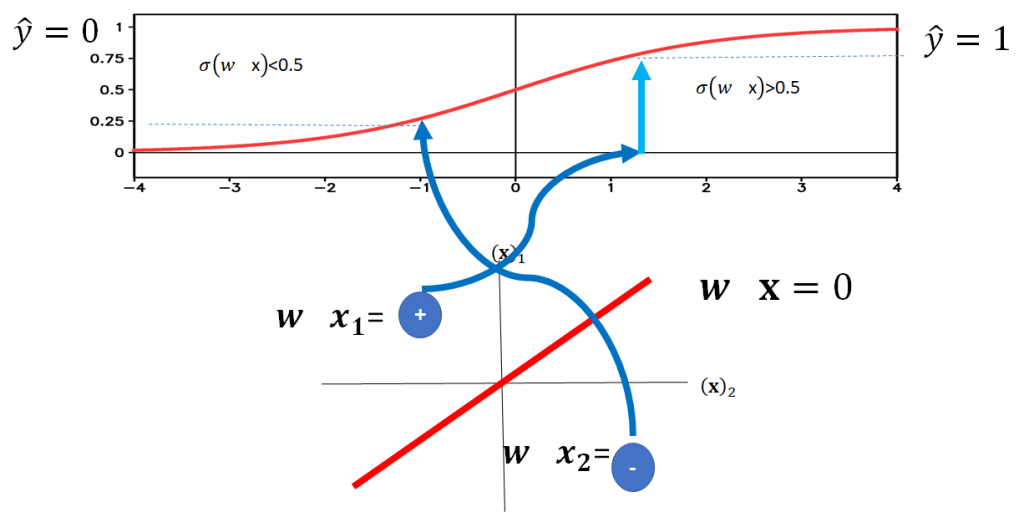
Now, lets use a logistic function then apply a threshold, first we can plug a negative value of z into the logistic function , if the value of the logistic function is less than 0.5 the output will $\hat{y}$ will be zero. Similarly, if the value of z is positive the value of the logistic function is grater than 0.5, if the value is larger then 0.5 , passing it through a threshold and we get a value of one for $\hat{y}$ .

*Fig 1*6 *Fig 15 line separating data this is where the decision surface insects with the plane where z equals zero, the sample* x₁ *is produces a positive value, this intern is passed to the logistic function* *that outputs a value larger than one half but less than one. The value of* x₂ is produces a negative value, when this is passed into the *logistic function* and get a number between zero and one, this is intern. passed through the. In both cases the value in passed between the threshold function .

We can also represent the logistic function as a probability. Consider the point x₁ the logistic function can be considered a conditional probability that $\hat{y}$ equals 0 or 1 given the sample of x₁. The probability $\hat{y}$ equals 1 give the sample x₁ is given by the following probability function $P( \hat{y}_1=1|\mathbf{x}_1, \mathbf{w},b)$ , we include the parameter vale $\mathbf{w}$ and $b$ to signify its dependent on the parameters or plane . Similarly as it is a probability mass function we can also determine the probability that $\hat{y}$ equals zero buy subtracting one:

$P( \hat{y}_1=0|\mathbf{x}_1, \mathbf{w},b)=1-P( \hat{y}_1=1|\mathbf{x}_1, \mathbf{w},b)$ ,

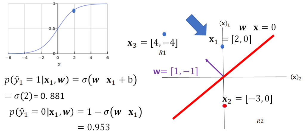
this is shown in Fig 17, as the point in on the side of the plane where $\hat{y}=1$ the $P( \hat{y}_1=0|\mathbf{x}_1, \mathbf{w},b)$ is smaller then $P( \hat{y}_1=1|\mathbf{x}_1, \mathbf{w},b)$

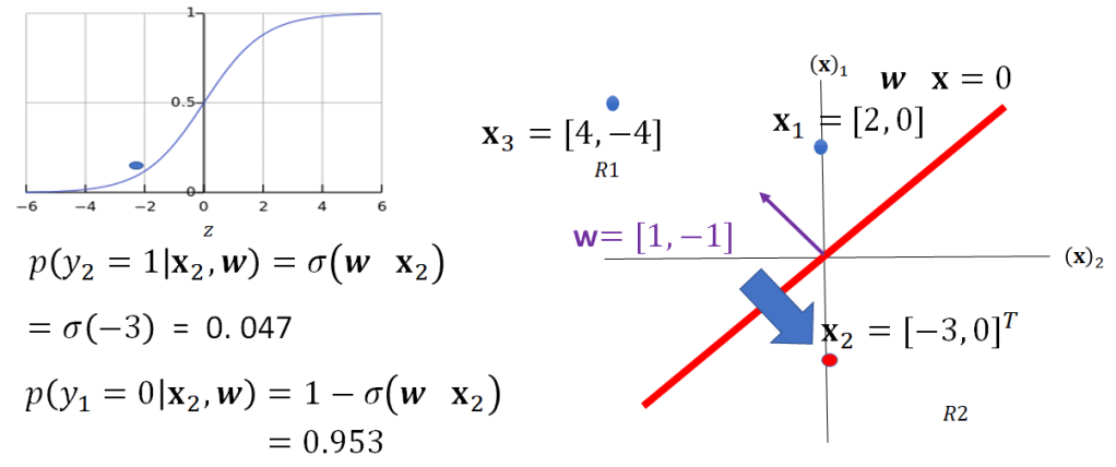
Similarly, we can calculate the value for x₂ this is shown in Fig 18, in this case because x₂ is on the other side of the plane corresponding to $\hat{y}=0$ the probability that $\hat{y}=0$ i.e $P( \hat{y}_1=0|\mathbf{x}_1, \mathbf{w},b)$ is larger than the probability that $\hat{y}=1$ $P( \hat{y}_1=1|\mathbf{x}_1, \mathbf{w},b)$ .

fig 18

To train linear classifiers we use Gradient Descent an optimization algorithm for finding a local minimum, in this case the minimum related to the number of misclassified samples, but this another story.

Linear Classifiers

Logistic Regression

Comments

Leave a comment Cancel reply

Linear Classifiers

Logistic Regression

Share this:

Comments

Leave a comment Cancel reply